Main concepts
Understanding pvfactors is simple. The pvfactors package builds on top of 3 distinct blocks
that allow a clear workflow in the calculation of irradiance, while keeping the complexity
separated for the different aspects of modeling. The schematics below shows what these three blocks are.
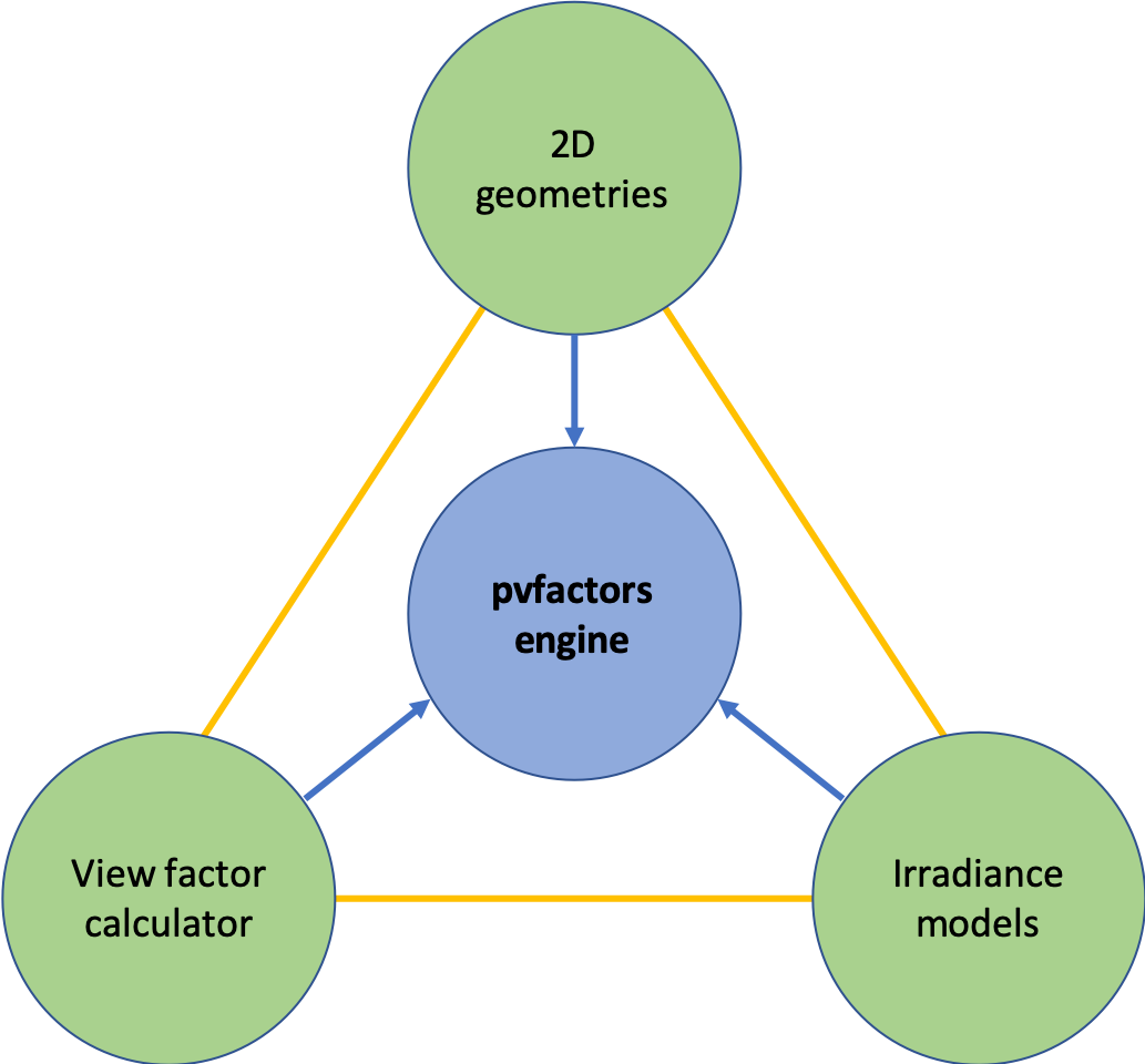
Fig. 1: The 3 building blocks of pvfactors
In pvfactors, everything starts with the 2D geometry of the PV array, and everything flows from there.
The user will use the geometry API to not only build the PV array geometry to be modeled, but also to get the results after the simulation.
A selected (or custom made) irradiance model can then be used to define the sky irradiance components that are incident on the surfaces. For instance in Fig. 2, the front surfaces of the PV rows are receiving direct sunlight, while their back surfaces aren’t receiving any. This is an example of what the irradiance model will define for all the surfaces.
A calculator can then be used to calculate a matrix of view factors between all the different surfaces.
Finally, these 3 blocks will be assembled together inside the pvfactors engine (see PVEngine) to solve the irradiance mathematical system described in the paper and in the theory section.
2D geometries
The main interface for building the 2D geometry of a PV array is currently the OrderedPVArray class. It can be used for modeling both fixed tilt and single-axis tracker systems on a flat ground. Here are some details on the concepts behind the OrderedPVArray class.
Note
For more information on how the geometry sub-package is organized, the user can refer to the detailed geometry API.
Understanding PV array 2D geometries
Let’s start with an example of a PV array 2D geometry plotted with pvfactors.
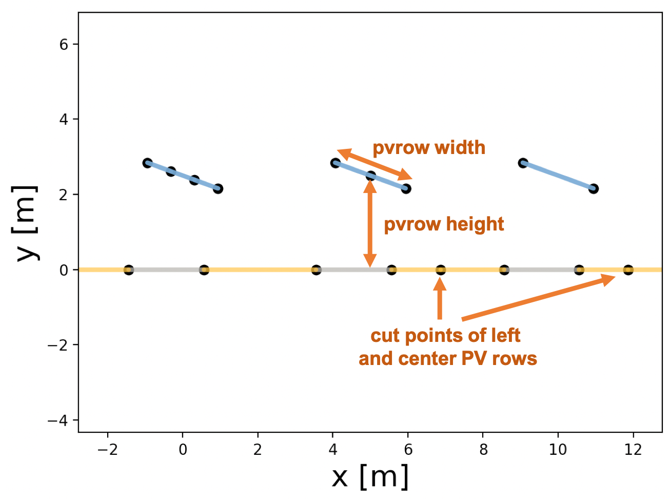
Fig. 2: Example of PV array 2D geometry in pvfactors
As shown in the figure above, a pvfactors PV array is made out of a list of PV rows (the tilted blue lines), and a ground (the flat lines at y=0).
The PV rows:
each PV row has 2 sides: a front and a back side
each side of a PV row is made out of segments. The segments are fixed sections whose location on the PV row side is always constant throughout the simulations, which allows the users to consistently track and calculate irradiance for given sections of a PV row side
each segment of each side of the PV rows is made out of collections of surfaces that are either shaded or illuminated, and these surfaces’ size and length change during the simulation because they depend on the PV row rotation angles and the sun’s position.
Note
In Fig. 2, the leftmost PV row’s front side has 3 segments, while its back side has only 1. And the center PV row’s back side has 2 segments, while its front side has only 1, etc.
The ground:
it is made out of shaded surfaces (gray lines) and illuminated ones (yellow lines)
the size and length of the ground surfaces will change with the PV row rotation and the sun angles. Physically, the shaded surfaces represent the shadows of the PV rows that are cast on the ground.
the ground will also keep track of “cut points”, which are defined by the PV rows (1 per PV row), and which indicate the extent of the ground that a PV row front side and back side can see.
Note
In Fig. 2, we can see 3 ground shadows, and the figure also shows 2 cut points (but there is a 3rd one located outside of the figure range on the right side).
PV array parameters
In pvfactors, a PV array has a number of fixed parameters that do not change with rotation and solar angles, and which can be passed as a dictionary with specific field names. Below is a sample of a PV array parameters dictionary, which was used to create the 2D geometry shown in Fig. 2.
pvarray_parameters = {
    'n_pvrows': 3,                            # number of pv rows
    'pvrow_height': 2.5,                      # height of pv rows (measured at center / torque tube)
    'pvrow_width': 2,                         # width of pvrows
    'axis_azimuth': 0.,                       # azimuth angle of rotation axis
    'gcr': 0.4,                               # ground coverage ratio
    'cut': {0: {'front': 3}, 1: {'back': 2}}  # discretization scheme of the pv rows
}
The tutorial section shows how such a dictionary can be used to create a PV array in pvfactors using the OrderedPVArray class. Here is a description of what each parameter means:
n_pvrows: is the number of PV rows that the PV array will contain. In Fig. 2, we have 3 PV rows.pvrow_height: the PV row height (in meters) is the height of the PV row measured from the ground to the PV row center. In Fig. 2, the height of the PV rows is 2.5 m.pvrow_width: the PV row width (in meters) is the cross-section width of the entire PV row. In Fig. 2, it’s the entire length of the blue lines, so 2 m in the example.axis_azimuth: the PV array axis azimuth (in degrees) is the direction of the rotation axis of the PV rows (physically, it could be seen as the torque tube direction for single-axis trackers). The azimuth convention used inpvfactorsis that 0 deg is North, 90 deg is East, etc. In the 2D plane of the PV array geometry (as shown in Fig. 2), the axis of rotation is always the vector normal to that 2D plane and with the direction going into the 2D plane. So positive rotation angles will lead to PV rows tilted to the left, and negative rotation angles will lead to PV rows tilted to the right.gcr: it is the ground coverage ratio of the PV array. It is calculated as being equal to the ratio of the PV row width by the distance separating the PV row centers.cut: this optional parameter is used to discretize the PV row sides into equal-length segments. For instance here, the front side of the leftmost PV row (always with index 0) will have 3 segments, and the back side of the center PV row (with index 1) will have 2 segments.
Irradiance models
The irradiance models then assign irradiance sky values like direct, or circumsolar components to all the surfaces defined in the OrderedPVArray.
Description
As shown in the full mode theory and fast mode theory sections, we always need to calculate a sky term for the different surfaces of the PV array.
The sky term is the sum of all the irradiance components (for each surface) that are not directly related to the view factors or to the reflection process, but which still contribute to the incident irradiance on the surfaces. For instance, the direct component of the light incident on the front surface of a PV row is not directly dependent on the view factors, but we still need to account for it in the mathematical model, so this component will go into the sky term.
A lot of different assumptions can be made, which will lead to more or less accurate results. But
pvfactors was designed to make the implementation of these assumptions modular: all of these assumptions can be implemented inside a single Python class which can be used by the other parts of the model. This was done to make it easy for users to create their own irradiance modeling assumptions (inside a new class), and to then plug it into the pvfactors PVEngine.
Available models
pvfactors currently provides two irradiance models that can be used interchangeably in the PVEngine and with the OrderedPVArray, and they are described in more details in the irradiance developer API.
the isotropic model
IsotropicOrderedassumes that all of the diffuse light from the sky dome is isotropic. It is a very intuitive assumption, but it generally leads to less accurate results.the (hybrid) perez model
HybridPerezOrderedfollows [1] and assumes that the diffuse light can be broken down into circumsolar, isotropic, and horizon components (see Fig. 3 below). Validation work shows that this model is more accurate for calculating back-side irradiance withpvfactors.
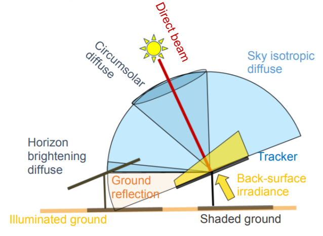
Fig. 3: Schematic showing direct and diffuse irradiance components on a PV system and according to the Perez diffuse light model [1]
View factor calculator
After creating a 2D geometry, the VFCalculator class can be used to calculate the view factors between all the surfaces of the array. A detailed description of what view factors are can be found in the theory section.
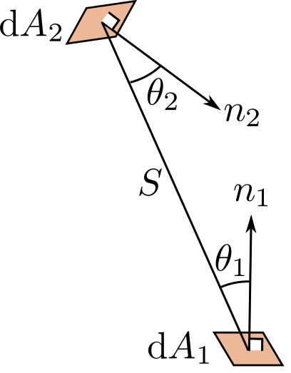
Fig. 4: The view factor from a surface 1 to a surface 2 is the proportion of the space occupied by surface 2 in the hemisphere seen by surface 1.
Next steps
get started using practical tutorials
learn more about the theory behind
pvfactorsdive into the developer API
Footnotes